
One-sided fractional Brownian Motion, introduced in , is an interesting class of Gaussian process, defined as a continuous moving average (CMA) of white noise:
$$ X_H(t) = \frac{1}{\Gamma(H + 1/2)} \int_{0}^{t} (t-u)^{H-1/2}\mbox{d} B_u, \tag{1}\label{eq:fbm}, $$
where \(B_u\) is the standard Brownian motion, and integration is understood in the mean-quadratic (Ito) sense for \(H>0\). This process has found important applications in electronics for modelling oscillatory noise , because its spectrum follows a power law.
This note presents a simple yet formal derivation of the fBM spectrum. The argument originally given in is somewhat complicated and leaves some gaps. The novel approach develops a handy closed-form formula using hypergeometric functions, establishing exact convergence rates of time-averaged spectra.
Since \eqref{eq:fbm} is nonstationary, we are going to use the Wigner-Ville instantaneous spectrum, which is the time-varying Fourier transform of the covariance with respect to the lag:
$$
S_X(t,\omega) = \widehat{F}_{\tau} \left[K_X\left(t-\frac{\tau}{2},t+\frac{\tau}{2}\right)\right](\omega)=\int K_X\left(t-\frac{\tau}{2},t+\frac{\tau}{2}\right) \mathrm{e}^{-\mathbf{i} \omega \tau} \mbox{d} \tau, \tag{2}\label{eq:spectrum}
$$
We easily find that the covariance of \(X=X_H\) in terms of time-difference coordinates equals
$$
K_X\left(t-\frac{\tau}{2},t+\frac{\tau}{2}\right)
= \frac{\left(t-\frac{|\tau|}{2}\right)^{H+\frac{1}{2}}\left(\frac{|\tau|}{2}+t\right)^{H-\frac{1}{2}}\,_2F_1\left(1,\frac{1}{2}-H;H+\frac{3}{2};\frac{2t-|\tau|}{2t+|\tau|}\right)}{\Gamma\left(H+\frac{1}{2}\right)\Gamma\left(H+\frac{3}{2}\right)} \tag{3}\label{eq:covariance}
$$
when \(|\tau| < t\), and is zero otherwise. Rather than directly transforming the covariance, we will be working with its second-derivative which happens to have a very simple form:
$$
\frac{\partial^2}{\partial t^2} K_X\left(t-\frac{\tau}{2},t+\frac{\tau}{2}\right) =
\frac{4^{2-H}t(4t^2-\tau^2)^{H-\frac{3}{2}}}{\Gamma\left(H-\frac{1}{2}\right)\Gamma\left(H+\frac{1}{2}\right)}\tag{4}\label{eq:covarianceD2}\cdot \mathbf{1}\{ |\tau| < 2 t \},
$$
and whose Fourier transform is easy to find in terms of the hypergeometric function \(_0F_1\)
$$
\widehat{F}_{\tau} \left[ \frac{\partial^2}{\partial t^2} K_X\left(t-\frac{\tau}{2},t+\frac{\tau}{2}\right) \right](\omega) = \frac{4\sqrt{\pi}t^{2H-1}\,_0F_1\left(;H;-t^2\omega^2\right)}{\Gamma(H) \Gamma\left(H+\frac{1}{2}\right)} \tag{5}\label{eq:covarianceD2_FT}.
$$
By taking the antiderivative twice, we find that the spectrum can be expressed in terms of \(_1F_2\):
$$
S_X(t,\omega) = \frac{2^{2H+1}t^{2H+1}\,_1F_2\left(H+\frac{1}{2};H+1,H+\frac{3}{2};-t^2\omega^2\right)}{\Gamma(2H+2)} \tag{6}\label{eq:covariance_FT}.
$$
The representation in \eqref{eq:covariance_FT} has the advantage that the \(_1F_2\) expression represents a smooth function which is easy to approximate. Using the theory of hypergeometric functions, we easily find that the instantaneous spectrum oscillates around \(\omega^{-2H-1}\):
$$S_X(t,\omega) = \omega^{-2H-1}\left(1-O\left(\frac{(t \omega)^{H-\frac{1}{2}}\left(\sin\left(\frac{\pi H}{2}-2t\omega\right)+\cos\left(\frac{\pi H}{2}-2t\omega\right)\right)}{\sqrt{2}\Gamma\left(H+\frac{1}{2}\right)}\right)\right) \tag{7}\label{eq:covariance_FT_approx}.
$$
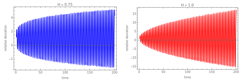
Despite these growing oscillations, we can prove that the running average converges and matches the power-law. Namely, when \(0<H<\frac{3}{2}\) we have the explicit formula
$$
\frac{1}{T}\int_{0}^T S_X(t,\omega)\ \mbox{d} t = \frac{2^{2H+1}T^{2H+1}\,_1F_2\left(H+\frac{1}{2};H+\frac{3}{2},H+2;-T^2\omega^2\right)}{\Gamma(2H+3)} \tag{8}\label{eq:covariance_FT_average},
$$
with the asymptotic behaviour
$$\frac{1}{T}\int_{0}^T S_X(t,\omega)\ \mbox{d} t = \omega^{-2H-1}\left(1+O_H(T\omega)^{H-\frac{3}{2}}\right), \quad T\omega \gg 1 \tag{9}\label{eq:covariance_FT_average_approx},
$$ demonstrating, for \(0<H<\frac{3}{2}\), the power law \(\omega^{-2H-1}\) as expected.
It should be noted that using the asymptotic expansion \eqref{eq:covariance_FT_approx} is insufficient to obtain the convergence rate in \eqref{eq:covariance_FT_average_approx}. This is because its second-order error term \(O((t\omega)^{H-3/2})\) does not capture oscillations, as seen with \(H=1/2\) resulting in an error term \(O(\log T / (T\omega))\).


