Iron logic defeats strawman

The straw man rhetorical technique is widely used: from scientific reviews (academia), through job interviews (industry) to the political discourse (international relations). The idea is simple: you distort arguments or opposing views to easier refute them. Not only is this trick popular, but proven successful statistically.

The best weapon against it is logically strict reasoning. Do not rush in quick answers and judgments, but rather use the playback and evaluate/falsify the claim in measurable terms as much as possible. This note aims to spread awareness of this logical fallacy and give illustrating examples, which appears particularly noteworthy in the context of the rise of misinformation.

  • Academia: a popular “straw man” variation is when reviewers exaggerate on English mistakes in scientific papers, concluding that the math content may be equally incorrect. While scientists should strive for perfection at the communication level, in life and computer sciences the technical content is more important. Fix English but don’t let your “this paper presents merit findings” claim get distorted by this. Remember that a) researchers compete with each other and b) it’s easier to complain on misspelled words than to evaluate complex math.
  • Industrial career: you believe you are a good fit, but the interviewers exaggerate on the necessity of some skill X which you don’t have at a moment. We speak of a fallacy when X is not essential for the role, or trivial to learn. Don’t let your “I am a good fit” get distorted!
  • International relations: instead of my own examples, I will refer to the excellent article written by the UK Defence Secretary. He attempts to falsify several claims coming from the government circles of the Russian Federation against the NATO alliance. One is “Russia being encircled by NATO”, which is replied by asking to measure the overlapping border.

Can Russia defend its economy from sanctions?

While western leaders are proud of imposing largest sanctions ever, it seems that Russia can withstand the crisis longer than some expect. The following two points, underrepresented in popular media, support this claim:

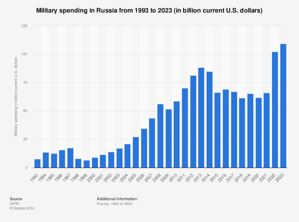
Russia seems both experienced and equipped to contain this crisis in short-term. After the crisis in 2014 it has used oil-generated income to collect more reserves and keep founding military.

Russian reserves in mln USD
Russian military spending in bln USD

But time will tell what the long-term financial consequences for the West and Russia would be.

Banks in Austria block financial help amid war on Ukraine

Amid the Russia’s invasion, some banks blocks money transfers to Ukraine. This effectively undermines the help efforts of both the international community and the expats. Here comes the wall of shame: a picture is worth thousand words:

Poland does the right thing: polish banks offered free transfers to Ukraine.

Demystifying TestDom

Recruiters nowadays use online timed tests when screening developers. I recently looked at Python & Algorithms Hard questions at TestDome. While the timing and hints seem to push towards implementing tricks from scratch, for the quality in long term it is better to structure the problem and use established solutions (divide & conquer). The battery of “hard” problems can be solved in few lines of code, using the standard Python libraries (Numpy, Pandas, Collections).

League Table (Hard)
The task is to essentially sort the football results by multiple criteria: first by the higher number of scores, next (breaking ties) by the lower number of games, finally (breaking ties) by the default order. While the hint suggests building a custom comparator, the effective way is by Pandas tables (5 lines).

import pandas as pd

def player_rank(self, rank):
        ts = []
        ts = map(lambda t:(t[1][0],t[1][1]['score'],t[1][1]['games_played'],t[0]),enumerate(self.standings.items()))
        df = pd.DataFrame(ts)
        df = df.sort_values(by=[1,2,3],ascending=[False,True,True]).reset_index()
        return df.loc[rank-1][0]

Sorted Search (Hard)
The task is to determine how many values in a sorted list are less than the given value. This is equivalent to finding the right position to insert (to maintain the sorted order). While the solution suggests playing with a variant of binary search on your own, the effective way is by the Python bisect algorithm (1 line).

from bisect import bisect_left

def count_numbers(sorted_list, less_than):
    return bisect_left(sorted_list,less_than)

Train Composition (Hard)
The task is to implement a data structure that mimics composing the train: one can quickly attach and detach to/from both ends. The effective way is to use Python double-ended queue (5 lines).

from collections import deque

class TrainComposition:
    
    def __init__(self):
        self.d = deque()
    
    def attach_wagon_from_left(self, wagonId):
        self.d.appendleft(wagonId)
    
    def attach_wagon_from_right(self, wagonId):
        self.d.append(wagonId)

    def detach_wagon_from_left(self):
        return self.d.popleft()
    
    def detach_wagon_from_right(self):
        return self.d.pop()

On Subgaussian Concentration of Missing Mass

The problem of missing mass goes back to the cryptographic work of Good and Turing during WWII, but has been also studied in the context of linguistic, ecology, and by probability theoreticians. The missing mass is defined as the weight of elements not observed in a sample, due to pure chance:

True and empirical frequency based on 100 samples, for Poiss(10).
The value of 12 is missing, and the corresponding bin is empty.

Such an event and the total mass of all unseen elements are exponentially small in the sample size.

Quite curiously, proving it rigorously has been quite hard. The first proof appeared at COLT’00, but has since then been reworked many times, in attempts to simplify and numerically improve. The arguments were based on a thermodynamic framework, logarithmic Sobolev inequalities and information theory. Formally, for some constant \(K>0\) we want

$$\Pr[\pm(M-\boldsymbol{E}M)>\epsilon]\leq \mathrm{e}^{-K\cdot n \epsilon^2}$$

where \(n\) is the sample size and \(M\) is the missing mass for the i.i.d. sample of size \(n\).

The problem of proving it “standard” concentration inequalities has been open so far. In reponse to this challenge, in my recent note I have proved it with Bernstein’s inequality, century old. So, no complicated approaches and refinements were necessary!

Approximating Tails of Beta Distribution

Beta distribution is ubiquitous in statistics, but particularly popular in real-world modeling. The beta-binomial model is perhaps the most known example, given the recent interest in Bayesian inference. But it was in use nearly 50 years ago, for example in toxicology.

Unfortunately, computing probabilities from the density depends on intractable incomplete beta integrals. This creates a demand for closed-form approximations, particularly for probability cfs/tails. The goal is to obtain an exponential concentration inequality in of Bernstein-type

$$\Pr[|X-\mathbf{E}[X]|>\epsilon]\leq \mathrm{e}^{-\frac{\epsilon^2}{2v^2+2c\epsilon}}.$$

Such bounds have been studied few times, the last one being the sub-gaussian approximation, that is when \(c=0\). Recently, I have further improved to optimal \(v\) (most important) and some good value of \(c\) (less important, but possibly worth further improvement). This gives a more accurate approximation when the distribution is very skewed (this happens when we model rare events, like conversion). For example with Beta(2,998) we get this:

The trick is to obtain a recursion scheme on central moments, and bound their growth by a geometric progression. The details are in my paper, and the code is shared in this notebook.

Improving State-of-Art on Sparse Random Projections

Random projections are widely used to reduce data dimension in various analyses. Provable guarantees were developed first in the important result of Johnson and Lindenstrauss on Lipschitz maps, but more recently there has been a lot of follow-up work in the context of machine-learning.

Particularly attractive are sparse random projections, which share similar guarantees as the original proposal, but are much faster to compute. In my recent paper I improve upon previous results of Meena Jagadeesan from NIPS’19. The key idea is to consider entropy of input data, a more fine-grained approach than in prior works. In the mathematical analysis I show this gives superior statistical guarantees. Besides that, the novel analysis seems to be cleaner and simpler.

The paper has been already reviewed and graded high at STACS’21, yet the committee members somehow didn’t want this machine-learning inspired topic in their program:

The PC members agreed that this is a non-trivial and interesting contribution. However, we had a very tough competition, and in the end, the PC members felt that the results were maybe too specialised for STACS audience

I am resubmitting it to a venue which will better appreciate the combination of ML and theory. I am also going to revisit this note and give a friendly overview of the work 🙂

Performance drawbacks of Tensorflow Datasets

Tensorflow, the popular framework for machine-learning, recommends its new dataset API for preprocessing and serving data. It supports useful tricks, such as caching data in memory, prefetching in parallel threads and others described in tutorials. Still, Tensorflow has issues with slow data slicing, so the dataset API may actually do harm in setups where computations are relatively fast; this includes linear models, word2vec and other shallow networks. In this note I illustrate this issue on training a classifier on MNIST dataset (handwritten images). As shown in the benchmark below, sometimes it makes sense to serve your data by custom generators not the recommended api.

The model is Logistic Regression. The loss function is implemented via logsumexp trick, for numerical stability and computational efficiency.

## model: Logistic Regression

w = tf.Variable(tf.random.normal(shape=(28*28,10),stddev=0.1),trainable=True)
optimizer = tf.optimizers.SGD(0.01)

@tf.function
def train_step(x, y):
  with tf.GradientTape() as tape:
    all_logits = tf.matmul(x,w) # (n_batch,n_class)
    y_logits = tf.gather(all_logits,y,batch_dims=1) # (n_batch,)
    logp = y_logits - tf.reduce_logsumexp(all_logits,axis=1)
    loss = -logp
  gradients = tape.gradient(loss,[w])
  optimizer.apply_gradients(zip(gradients,[w]))

Now we compare two ways of serving the data: by custom generators and by Dataset API (with caching and prefetching for better performance).

## serving data: a) via custom generator b) via TF Dataset API

def gen_batch(X,n_window):

  def gen():
    for i in range(0,len(X),n_window):
      yield X[i:i+n_window]
  
  return gen

def gen_data():
  n_window = 32
  return zip(gen_batch(x_train,n_window)(),gen_batch(y_train,n_window)())

tf_data = tf.data.Dataset.from_tensor_slices((x_train,y_train))
tf_data = tf_data.batch(32,drop_remainder=True)
tf_data = tf_data.cache()
tf_data = tf_data.prefetch(1)

Below running the comparison, the graph and dataset are warmed by one full-pass (then the graph gets built and the api pipeline is cached). Both approaches fit the same classifier, but the code with custom generator runs 50% faster. For the full code, see the jupyter notebook.